How the loader draws the dot-based Saturn in Elite's epic loading screen
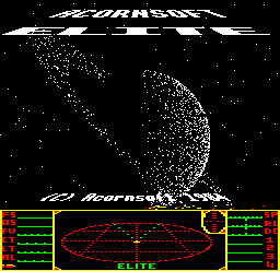
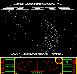
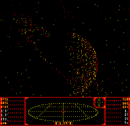
The original Elite oozes quality from the very start - before the game has even loaded, even. For those of us who were lucky enough to experience Acornsoft Elite when it came out, the game's loading screen was a revelation, because after the familiar Acornsoft loading screen has announced the game's name, the real magic of Elite takes over with this thing of beauty:
It's hard to overstate how important this screen was back in the day, particularly to those of us on simpler systems. Loading Elite from cassette is an exercise in patience, as it takes several minutes for the game to load, but our reward is the Saturn loading screen. Sure, owners of disc drives also get to see the Saturn loading screen, but for them it only appears for a few seconds, while those of us in the cheap seats get to stare at it for what seems like eternity, watching the cassette blocks counting up.
The anticipation is real, and the Saturn screen makes it pretty clear that this game will be worth the wait. Let's see how Saturn gets its solid 3D feel and those beautiful rings.
Three-stage Saturn
------------------
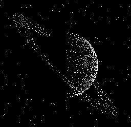
This deep dive covers the drawing of the Saturn planet, its rings, and the background stars. If you take away the dashboard and title images from the loading screen, you can see Saturn in all its glory, hanging there rather magnificently in the dimly lit depths of space:
The drawing is done in three stages, with the planet being drawn by part 1 of PLL1, the stars by part 2, and the rings by part 3. Note that the 3D text on the loader screen is not described here, but these are simply static images that are loaded in part 3 of the loader.
The positions of the dots in the loading screen are generated by Elite's pseudo random-number generator (see the deep dive on generating random numbers for details). This random number generator is seeded at the start of the PLL1 routine to a value from the 6522 System VIA T1C-L timer, which will be pretty random, so the exact distribution of dots drawn differs slightly each time the game loads. (Though this isn't true for the Master's loading screen, as it isn't seeded properly - see the end of this article for details.)
Generally speaking, each of the three stages draws a scattering of random points, uniformly chosen across the whole screen, which are then passed through a "filter" that acts a bit like a cardboard cut-out, in that the filter only shows those points which lie inside specific chosen regions of the screen. These specific regions are the planet's rings, the planet's disk, or the background area of stars. For example the filter for the background stars only plots dots which are outside of the planet's circular disk.
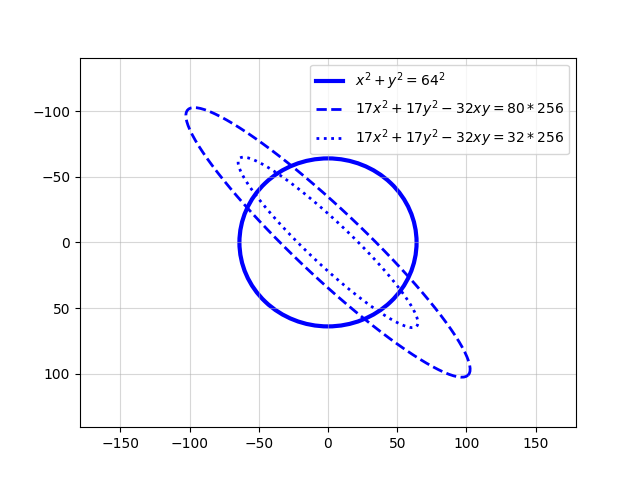
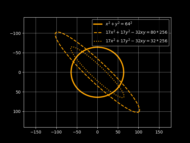
Each region of the screen is identified by one or more boundary, each with its own equation, illustrated here:
The routine is split into three parts, so let's look at each of them in turn, starting with the background stars.
The background stars (part 2 of PLL1)
-------------------------------------
Let's start with part 2 of PLL1, which draws the background stars, as this is the easiest routine to describe (the planet is drawn first in part 1, but we'll describe that later).
The stars are drawn by randomly choosing pixels uniformly across the screen, and then only plotting them if they lie outside of the planet's disk equation.
So, for each star, we draw a pixel at (x, y) where:
  x = a signed random number from -128 to 127

  y = a signed random number from -128 to 127
and where:
(x^2 + y^2) DIV 256 > 17
The final equation here rearranges into:
x^2 + y^2 > 65.96^2
which is the filter that ensures each star is outside of the planet's circular disk. It actually ensures the stars are slightly further outside of the planet than the planet's exact radius (hence the use of 65.96^2 in place of 64^2), so this emulates a thin dark atmospheric ring, surrounding the planet, in which no stars are drawn. This atmospheric gap is only 2 pixels wide, so is barely noticeable.
The logic that checks (x^2 + y^2) DIV 256 > 17 uses the square routine at SQUA2, which assumes x and y are signed numbers (i.e. in the range -128 to 127). However, when the pixels are finally drawn to the screen, they are treated as unsigned quantities (i.e. ranging from 0 to 255). This effectively adds 128 to x and y, which means the coordinates are plotted relative to an origin at the centre of the screen. This trick, of using unsigned bytes to shift the graphics origin to the centre of the screen, is used in all of the stages in the Saturn loader screen.
To see this process in action, check out this BBC BASIC demonstration of the star-drawing algorithm (link opens in a new window). This uses the Owlet engine to run the BASIC program in your browser.
Saturn's rings (part 3 of PLL1)
-------------------------------
Part 3 of PLL1 is responsible for plotting the rings. In this part of the algorithm, dots are drawn if they lie inside an outer ellipse, outside an inner ellipse, and not behind the planet. You can see the two ellipses in the diagram from above, repeated here:
First, we choose random numbers r5, r6:
  r5 = a signed random number from -128 to 127

  r6 = a signed random number from -128 to 127
Then let:
r7 = r5 DIV 4
Next, convert r6 and r7 into screen coordinates by a transformation:
  x = r6 + r7

  y = r6
This transformation from r5, r6 and r7 to x and y sets (x, y) to be any point along a wide diagonal band running from the top-left of the screen to the bottom-right of the screen. This can be seen because the above equations can be written as:
y = x - r5 DIV 4
This transformation to a wide diagonal band concentrates the candidate points so that they are more likely to lie within the planet rings, compared to a random point chosen anywhere over the entire screen, which is more likely to miss the planet rings entirely, and waste CPU time. So this transformation makes the code faster. Another benefit is that if r5 > 0, then the point (x, y) lies in the upper-right triangle of the screen, i.e. behind the planet. This logic is used later on, to avoid drawing the rear rings as they pass behind the planet.
Next we apply the elliptical filter, to ensure that (x, y) lies between the two ellipses shown in the diagram above. This is implemented in the code by checking:
32 <= ((r6 + r7)^2 + r5^2 + r6^2) / 256 < 80
Note that this rearranges into:
  32 * 256   <=   x^2 + (4 * r7)^2 + y^2               <   80 * 256

  32 * 256   <=   x^2 + 16 * (x - y)^2 + y^2           <   80 * 256

  32 * 256   <=   x^2 + 16 * (x^2 - 2xy + y^2) + y^2   <   80 * 256

  32 * 256   <=   17 * x^2 - 32xy + 17 * y^2           <   80 * 256
Note that an equation of the form:
  ax^2 + bxy + cy^2 = 1

  with a > 0, c > 0 and b^2 - 4ac < 0
is a general ellipse, centred on the origin (see this Wikipedia article on general ellipses for details). The equations:
17 * x^2 - 32xy + 17 * y^2 = 32 * 256
and:
17 * x^2 - 32xy + 17 * y^2 = 80 * 256
represent the inner and outer ellipse boundaries of the planet rings (as shown in the diagram above). Hence the above filter is checking that (x, y) lies inside the outer ellipse, and outside the inner ellipse - i.e. in the ring shape between the two ellipses.
On top of this, the code makes additional filter checks to ensure that the rings are not drawn when they pass behind the planet. These filters check whether either:
(x^2 + y^2) / 256 >= 16 (the point is outside the planet's disk)
or both these are true:
  (x^2 + y^2) / 256 < 16        (the point is inside the planet's disk)

  r5 < 0                        (and the point is on the rings that go
                                 in front of the planet)
If the candidate point (x, y) passes all of the above checks, then it must lie in a visible part of the rings, and so is plotted. Note that there is a slight inconsistency in the code here - the rings do not get obscured by the 2-pixel wide mathematical atmosphere that the background stars are obscured by. This could be a slight oversight by the Elite authors?
Again, when they are plotted on the screen, the values (x, y) are treated as unsigned quantities, which effectively adds 128 to each of them.
To see this process in action, check out this BBC BASIC demonstration of the ring-drawing algorithm (link opens in a new window). This uses the Owlet engine to run the BASIC program in your browser.
The planet (part 1 of PLL1)
---------------------------
The planet-drawing routine in part 1 of PLL1 draws the dots inside the planet's disk. We describe this routine last because it is the most complicated of the three routines, as it plots the dots with a non-uniform probability distribution. This ensures that the dots are clustered nicely on the right-hand side of the planet, giving the planet the illusion of being a solid 3D sphere.
First, we pick two uniform random numbers:
  r1 = a signed random number from -128 to 127

  r2 = a signed random number from -128 to 127
Next, we check that the point (r1/2, r2/2) lies inside the planet's disk, i.e. that:
(r1^2 + r2^2) < 128^2
By using r1/2 and r2/2 here (in place of r1 and r2) and by doubling the circle radius to 128, we increase the number of random coordinates that intersect the circle of interest, which speeds things up. Another advantage of doing this is that it gives us an extra bit for numerical accuracy. The final circle shown, though, is still a circle of radius 64, since:
(r1^2 + r2^2) < 128^2
is algebraically equivalent to:
x^2 + y^2 = 64^2
if we substitute (x, y) for (r1/2, r2/2).
Next, we choose screen coordinates as follows:
  y = r2

  x = SQRT(128^2 - (r1^2 + r2^2))
We then plot a point at (x/2, y/2) using unsigned coordinates, which shifts the origin to the centre of the screen (as with the stars and rings).
To see this process in action, check out this BBC BASIC demonstration of the planet-shading algorithm (link opens in a new window). This uses the Owlet engine to run the BASIC program in your browser.
Let's now take a look at that clever SQRT calculation, which, incredibly, packs a whole probabilistic 3D lighting model for the shaded planet sphere, all into this single line.
Probability distribution for planet shading
-------------------------------------------
The final line of code above:
x = SQRT(128^2 - (r1^2 + r2^2))
does a particularly neat mathematical transformation, changing the probability distribution for each point (r1, r2) from being uniformly scattered across the planet's disk, into a scattering of points which correctly obey the lighting model for a sphere illuminated from the right-hand side. It does this using the SQRT function to calculate a square root, as implemented by the ROOT routine.
Intuitively, the SQRT function used here always returns a positive number, so it shifts all lit points to the right-hand side of the planet, as seen below. Also, the SQRT function "squishes" the distribution of the points, so that they are more clustered towards the right-hand rim of the planet. In effect the SQRT changes the probability distribution of points from "uniform", to one which is more concentrated towards the right-hand rim of the planet's disk.
So whereas the initial points (r1, r2) were scattered uniformly across the circular planet, after passing through the SQRT function, we obtain transformed points (x, y) that are scattered non-uniformly across the circular disk. The idea is illustrated here:
If we focus on one particular y-coordinate of the planet's disk (illustrated above as the right-hand red rectangle), then the points scattered along it have more probability of appearing towards the right. In this sense, the probability is "distributed" more towards the right than towards the left. Mathematically, the probability of a point appearing at a given x-coordinate along the red rectangle is called the "probability density function" (PDF), illustrated here:
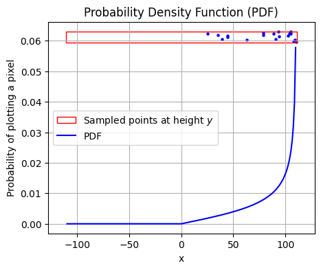
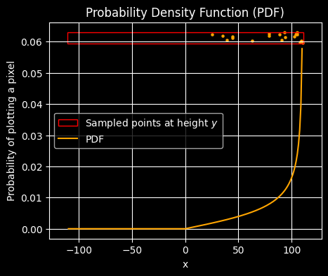
Note that even though the points themselves are scattered and lumpy, the underlying PDF curve is a smooth mathematical function, i.e. not at all lumpy. But this raises the questions, what is the exact formula for the PDF shown above, and why or how does this make the nice effect of an illuminated 3D sphere?
Note that modern computer languages often include random-number generating functions which return non-uniform probability distributions (e.g. Gaussian or Normal distributions). How do they do this? Just like Elite's Saturn planet code, they usually start with a uniform random number, u say, and squish it a bit to change it into the probability distribution that they want. The formal theory behind changing one probability distribution into another one in this way is called "Inverse transform sampling" (see Wikipedia for details). From this theory, if you want to change a uniform random number u (in the range 0 to 1) into your desired probability density function, then you push u through the squishing function:
x = CDF-1(u)
where CDF-1 denotes the inverse of the cumulative density function (CDF) for your target PDF. (Note that a CDF is defined to be the integral of its corresponding PDF.) This makes the output variable x be a random number in the distribution given by the desired PDF.
Remember, the formula that Elite uses to generate x is:
x = SQRT(128^2 - (r1^2 + r2^2))
So that's its squishing formula. This can be rewritten as:
  x = SQRT(rx^2 - (128u)^2)

  u = |r1 / 128|

  rx = SQRT(128^2 - y^2)
where:
- u is a uniform random number between 0 and 1 or x / 128 (note that due to the filtering of r1^2 + r2^2 < 128^2, u = |r1 / 128| will generally be less than 1, but this does not affect the explanation that follows)
- rx is the x-coordinate of the right-hand side of the planet's circle at height y = r2, i.e. the x-coordinate of the right-hand side of the red rectangle shown in the above diagram (assuming the origin (0, 0) is taken to be the centre of the circle)
From the theory of Inverse Transform Sampling, the squishing function:
x = SQRT(rx^2 - (128u)^2)
is the inverse cumulative density function (CDF-1) of the probability distribution that we seek to find. So therefore, to recover the CDF from this, we have to invert the function, i.e. solve it for u. Doing this gives:
u = SQRT(rx^2 - x^2) / 128 = CDF(x)
Next, to convert this cumulative distribution function (CDF) to a probability density function (PDF), we differentiate it, since a CDF is defined to be the integral of a PDF. The derivative of:
y = SQRT(rx^2 - x^2) / 128
with respect to x is:
  dy/dx = x / (SQRT(rx^2 - x^2) * 128)

        = x / (SQRT(128^2 - y^2 - x^2) * 128)
So this is the PDF that describes x, when x > 0:
pdf(x) = x / (SQRT(128^2 - y^2 - x^2) * 128)
When x < 0, just by knowing that the original SQRT line of code always gives a positive output, we can say that pdf(x) = 0, when x < 0.
Phew!
Interpreting the probability distribution geometrically
-------------------------------------------------------
Now we know that for x > 0, the transformed probability distribution is:
pdf(x) = x / (SQRT(128^2 - y^2 - x^2) * 128)
So how can we interpret it geometrically?
The PDF derived above can be rewritten as:
pdf(x) = x / 128z
since for the 3D sphere, x^2 + y^2 + z^2 = 128^2, and so:
z = SQRT(128^2 - y^2 - x^2)
Now suppose that P is the point on the sphere with coordinates (x, y, z), and the centre of the sphere is at O = (0, 0, 0). If nx, ny and nz are the 3D components of a unit-normal vector n pointing up from the sphere's surface, then the vector OP = [x y z] is parallel to the vector n = [nx ny nz], as n is effectively a continuation of OP from the surface into space. If two vectors are parallel, then one must be a multiple of the other, so we have:
  [ x ]          [ nx ]
  [ y ]  =  k' * [ ny ]
  [ z ]          [ nz ]
for some scalar k'. So therefore we have:
  pdf(x) = x / 128z

         = (k' * nx) / (128 * k' * nz)

         = nx / 128nz
Hence the PDF can be rewritten as:
pdf(x) = k nx/nz
where k = 1 / 128.
If we have Cartesian unit vectors i, j, k in the x, y, z directions, and n is the unit normal vector from the sphere's surface, then:
nx = n.i = cos(theta_x)
where theta_x is the angle the sphere's unit normal makes with the x-axis. This follows from:
(nx, ny, nz).i = nx
and also from the definition of the vector dot product:
  n.i = |n||i|cos(theta_x)
      = cos(theta_x)
since n and i are both unit vectors.
Also, by exactly the same reasoning as above, but for z in place of x, we also have:
nz = n.k = cos(phi_z)
where phi_z is the angle the sphere's unit normal makes with the z-axis.
Hence the probability distribution for drawing a point at (x, y) is proportional to cos(theta_x) / cos(phi_z), or:
pdf = k cos(theta_x) / cos(phi_z)
where theta_x is the angle the sphere's normal vector makes with the x-axis (i.e. the direction the light source is coming from), and phi_z is the angle the sphere's normal vector makes with the z-axis (i.e. the angle we are viewing from), and k is a constant of proportionality.
The Saturn planet's lighting model
----------------------------------
The planet's surface is modelled as a diffusely reflecting surface, i.e. having a perfectly matt texture. This means that each point on the planet's surface scatters light equally in all directions. This is known as Lambertian reflectance in computer graphics (see this Wikipedia article for further details).
The numerator of the (geometrically interpreted) PDF expression, i.e. cos(theta_x), calculates how much light intensity is received at that point of the planet's surface. All of this light is assumed to be diffusely reflected (under the assumption of Lambertian reflectance). The amount of light captured at the surface, and hence the amount of light diffusely reflected, is simply the cosine of the angle between the light source (from the right) and the sphere's unit normal vector.
The more square-on the surface normal is to the light source, the more light is received, and hence scattered from that point. For example, if the surface normal points directly towards the light source (so theta_x = 0), then we have cos(theta_x) = 1, indicating that 100% of the light is received and scattered from this point. The more tilted the unit normal is to the light source, the less light is incident to that point. For example, if the surface normal points at 90 degrees to the light source (so theta_x = 90), then we have cos(theta_x) = 0, indicating that 0% of the light is incident to that point, and hence zero light is scattered from this point.
The denominator of this expression, i.e. cos(phi_z), calculates the amount of "compression" that a grid of dots would experience if it was angled to the viewer's line of sight by angle phi_z. This is like a visual compression that texture-mapped computer graphics go through, if the image is angled away from the line of sight. Intuitively, if a sheet of paper was covered in random dots, with N dots per square cm on the page, and we tilt the page at an angle phi_z to the viewer's line of sight, then the page's apparent width will be compressed by a factor of cos(phi_z), and so the dot density the viewer sees increases by a factor 1/cos(phi_z). That is what the denominator in this transformed PDF is doing!
As the PDF for plotting a point at (x, y) is:
pdf = k cos(theta_x) / cos(phi_z)
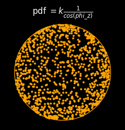
where k is a constant of proportionality, we can investigate the relative merit of the denominator and numerator visually. For example, if we only had the numerator present, then the plot would look like this:
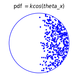

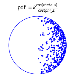
Whereas if we have the denominator present only, then we get the texture-mapping effect only. Here you can see the points are more clustered towards the outside of the circle, which (with the assistance of a little imagination) shows a slight 3D curvature:
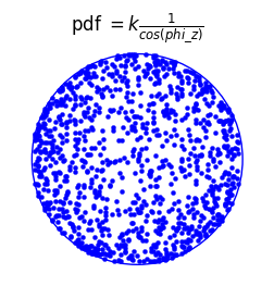
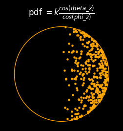
But if we have both the numerator and denominator present, then we combine the above two effects, and get a more three-dimensional looking sphere:
So we've seen that within this single SQRT calculation, there really is a probabilistic 3D lighting model, which includes a probability density transform, a 3D sphere with Lambertian reflectance, and also some texture mapping, just to cap it all off. This is yet is another particularly elegant piece of mathematics and programming by the Elite authors. Does this single line rival the notorious brilliance of the Quake inverse-square root algorithm? I like to think so.
Variations of the Saturn loader screen in different versions of Elite
---------------------------------------------------------------------
The Saturn-drawing algorithm in the PLL1 routine is identical in all versions of Elite. However, there are some subtle differences:
- The BBC Micro cassette and Electron versions have up to 1280 dots in the planet, while the BBC Micro disc, Master and 6502SP versions have up to 768 - this is set by the CNT variable. See the CNT code comparison for details.
- The BBC Micro cassette and Electron versions have up to 1280 dots in the rings, while the BBC Micro disc, Master and 6502SP versions have up to 819 - this is set by the CNT3 variable. See the CNT3 code comparison for details.
- The Master version fails to seed the random number generator properly, so in that version Saturn's dots are always identical; all the other versions grab a seed value from the System VIA timer, so they are different every time. See the PLL1 part 1 routine comparison for details.
So the Electron and cassette versions are actually more complex than the later ones, which is unexpected, and there are various bits of copy protection code inserted into the routine, which differ between versions, but they don't affect the planet. You can see these in all three routine comparisons: part 1, part 2 and part 3.
If you compare the results side by side, the number of dots is quite clearly different. For example, here's the cassette version:
and here's the disc version:
The Master version also fails to set the palette correctly, so the dashboard remains a mess, which is a bit of a shame; here's what it looks like:
All this variety helps make the Elite loading screen one of the most interesting bits of code in the whole game, and that's really saying something...